backpropagation using random feedback weights

You probably know the backprop algorithm by heart. You may also have good intuitions about why it works, and why it is the way it is. I certainly thought so, until I came across a paper by Timothy P. Lillicrap et al. with a rather counter intuitive claim that using random weights during the backward pass of backprop algorithm works just as well as using the actual network weights! This went against my intuition of backprop, so I decided to do a series of experiments to examine it. My code is available for anyone who wants to play around with it.

Backpropagation refresher

Let’s take a refresher on how backprop works by diving straight into the math, specifically the part that is affected by using random weights. The three equations below (which I have liberally taken from Wikipedia) describe the backward pass of the backprop algorithm.

\[\begin{gathered} {\frac {\partial E}{\partial w_{ij}}}=o_{i}\delta _{j} \\ \Delta w_{ij}=-\eta {\frac {\partial E}{\partial w_{ij}}}=-\eta o_{i}\delta _{j} \\ \delta _{j}={\frac {\partial E}{\partial o_{j}}}{\frac {\partial o_{j}}{\partial {\text{net}}_{j}}}={\begin{cases}(o_{j}-t_{j})o_{j}(1-o_{j})&{\text{if }}j{\text{ is an output neuron,}}\\{\color{green}\sum _{\ell \in L}\delta _{\ell }w_{j\ell }}o_{j}(1-o_{j})&{\text{if }}j{\text{ is an inner neuron.}}\end{cases}} \end{gathered} \]

The first equation tells us how to calculate the change in Error \(E\) as we change a weight \(w_{ij}\) in the network. \(o_{i}\) is the output of sigmoid activation function (In this post we have assumed activations are sigmoid). The second equation calculates the amount that the weight needs to be adjusted \(\Delta w_{ij}\). It simply multiplies the partial derivative from the first equation by the learning rate \(\eta\). The (-) sign is there so the adjustment of the weight is in the direction of decreasing \(E\).

So far easy peasy, because the juicy part is hiding in the calculation of \(\delta \). It has two terms: \(\frac {\partial E}{\partial o_{j}}\) and \(\frac {\partial o_{j}}{\partial {\text{net}}_{j}}\). You can see \(\delta \) is calculated differently for the output layer than the hidden(inner) layers. The \(\frac {\partial o_{j}}{\partial {\text{net}}_{j}}\) is the same for both output and hidden layers. It is the \(o_{j}(1-o_{j})\) that you see on the right hand side which is the derivative of our sigmoid activation function.

The part that is different, is the calculation of \({\frac {\partial E}{\partial o_{j}}}\). It is pretty obvious for the output layer neurons; It is simply the difference between output and target \(o_{j}-t_{j}\) (given that squared error is used to calculate\(E\) ).

Calculation of \(\frac {\partial E}{\partial o_{j}}\) gets more interesting for a hidden layer neuron (the part in \({\color{green}green}\)). That is where the “propagating backward” of the backpropagation algorithm happens. Let’s look at it more closely and understand why it looks the the way it does.

At first, the term \(\sum _{\ell \in L}\delta _{\ell }w_{j\ell }\) may seem to have been pulled out of a hat. Let’s see if we can derive it from scratch for the network below:

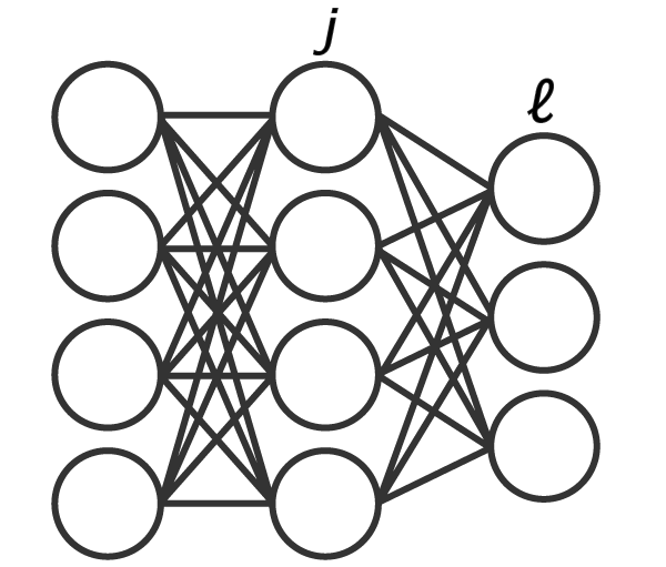
We write the squared error first: \[ E={\tfrac {1}{2}}\sum _{\ell \in L}(t _{\ell}-o_{\ell })^{2}\]

Now let's replace \(o_{\ell }\) with \(\sigma (o_{j\ell }w_{j\ell})\) \[ E={\tfrac {1}{2}}\sum _{\ell \in L}(t_{\ell}-\sigma (o_{j}w_{j\ell}))^{2} \]

Now we can take the derivative of \(E\) w.r.t. \(o_{j}\). We will have to use chain rule three times. (Each term in the chain rule is colored differently for clarity) \[{\frac {\partial E}{\partial o_{j}}}=\sum _{\ell \in L}{\color{red}(t _{\ell} - \sigma (o_{j}w_{j\ell}))}{\color{blue}\sigma (o_{j}w_{j\ell})(1 - \sigma (o_{j}w_{j\ell}))}{\color{green}w_{j\ell}} \]

If you look closely, you'll see: \[\begin{aligned} {\color{red}(t _{\ell} - \sigma (o_{j}w_{j\ell}))}{\color{blue}\sigma (o_{j}w_{j\ell})(1 - \sigma (o_{j}w_{j\ell}))} \\ == {\color{red}(t_{\ell}-o_{\ell })}{\color{blue}o_{\ell}(1-o_{\ell})} \\ == {\color{purple}\delta _{\ell}} \end{aligned}\]

Therefore: \[{\frac {\partial E}{\partial o_{j}}} = \sum _{\ell \in L} {\color{purple}\delta _{\ell}} {\color{green}w_{j\ell}} \]

Now with that out of the way let get to the experiment.

Experiment setup

To compare the result of regular backpropagation to backpropagation using random feedback, my code repeats the training-testing cycle 30 times and the results are used for a statistical significant test. In each experiment:

• I trained and tested two identical networks for 200 epochs on MNIST dataset, 30 times.

• Each time starting from a new set of random weights (w1, w2, and w2_feedback) and new random samples from MNIST for training and testing.

• Both networks had the same learning rate of 0.07 which was tuned to get the best performance for regular backprop.

• w2_feedback is scaled up logarithmically with each epoch. This is where I deviate from the paper. I found that this results in faster convergence.

• The initial w1(input to hidden) and w2(hidden to output) were identical for both networks.

• Both networks are two layers with 784 input (28x28 pixel image) and 10 output units (0 to 9 digits). I experiment with different number of units in the hidden layer.

• The only difference between the two networks is that I used normally distributed random weights (w2_feedback) during backprop. w2_feedback is the \(\color{green}w_{j\ell}\) in our equations above. Normally the same weights are used during forward and backward pass. Here we used a random \(w_{j\ell}\)(w2_feedback in the code) in the backward pass.

• w2_feedback remained constant during training.

• After each training-testing run, accuracy was measured and recorded on the test set.

After 30 runs, t-test is performed on recorded accuracies of each run to see if there is a significant difference in performance. Results are reported in the table below.

Results

hidden units	training set size	test set size	avg. accuracy w/ normal Backprop	avg. accuracy w/ random feedback Backprop	t-test p value	# of runs
20	50k	10k	90.0%	93.5%	0.003	30
40	50k	10k	96.1%	96.0%	0.027	30

It's pretty surprising that backprop with random feedback weights learns as well as vanilla backprop! In the case of 20 hidden units, it performs even better. Here are some sample loss plots from training-testing cycles.

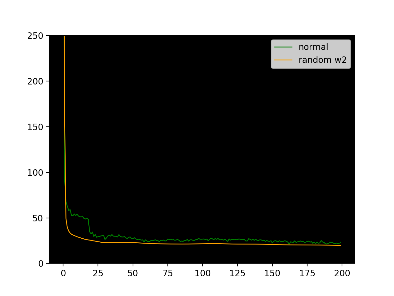
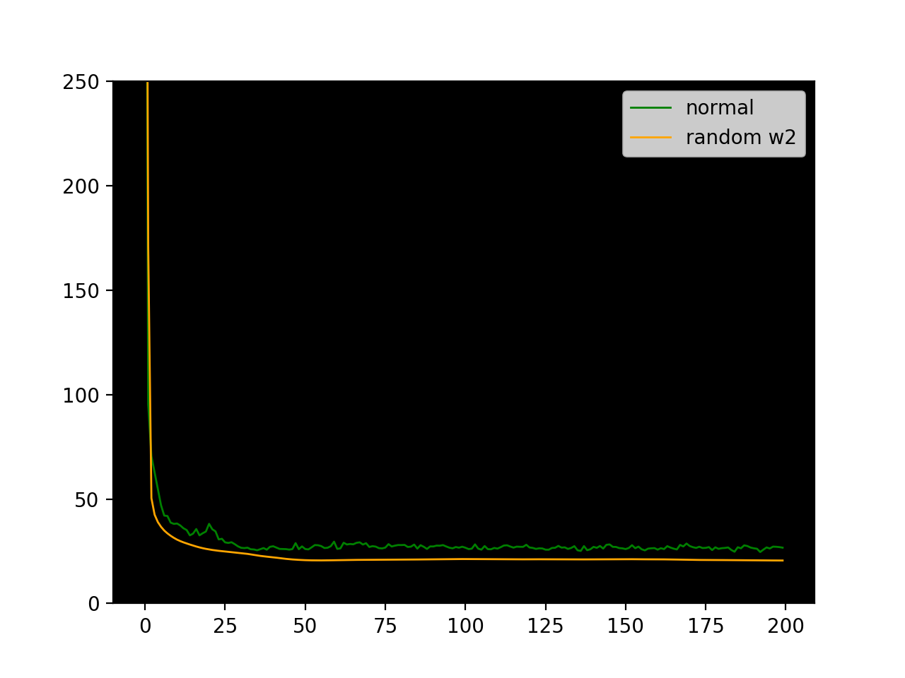
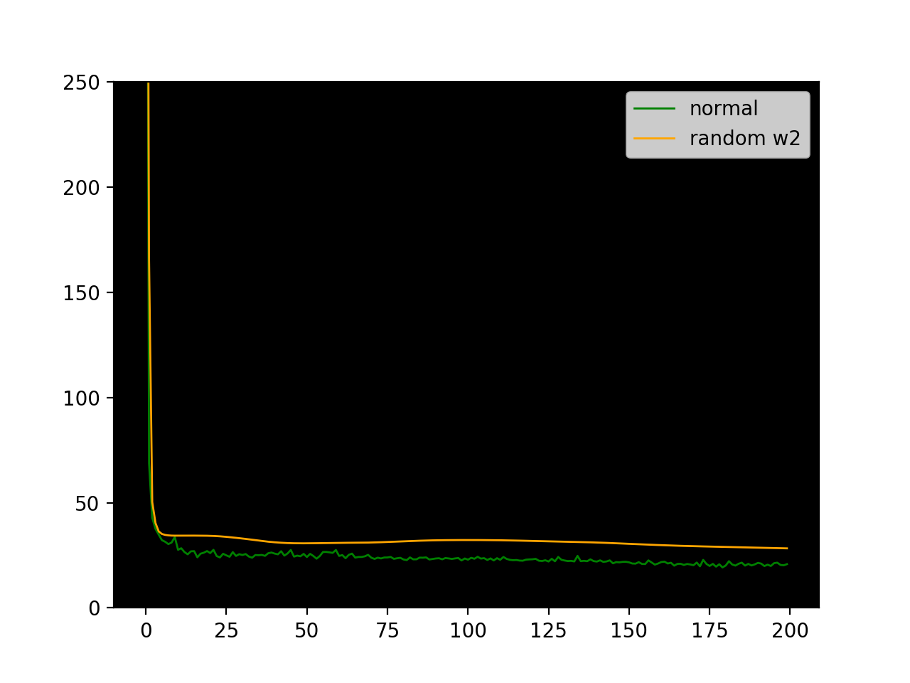
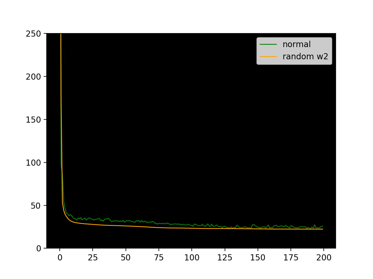
Interestingly the loss plot for the random w2_feedback is much smoother.

I’m surprised not more people are talking about this. It seems like backpropagation is taken for granted. I feel like this should open a new degree of freedom in designing new models, and we should be able to exploit it somehow.

Post experiment soul searching

But why this result? I had an intuition that by using a random but fixed w2_feedback during backprop, neurons in the hidden layer learn their incoming weights (w1) to minimize the \(\delta _{\ell}\) of neurons in the output layer that they happen to have a high outgoing weight to. This kind of explains why the network is still able to learn. Each neuron in the hidden layer is predetermined to fit to a specific output neuron by the random selection of feedback weights.

This hypothesis predicts that the correlation between the feedforward w2 and w2_feedback should increase as we train. So to test it, I measured and ploted that correlation. The figure below also plots the Pearson Correlation between w2 and w2_feedback as w2 is learned.

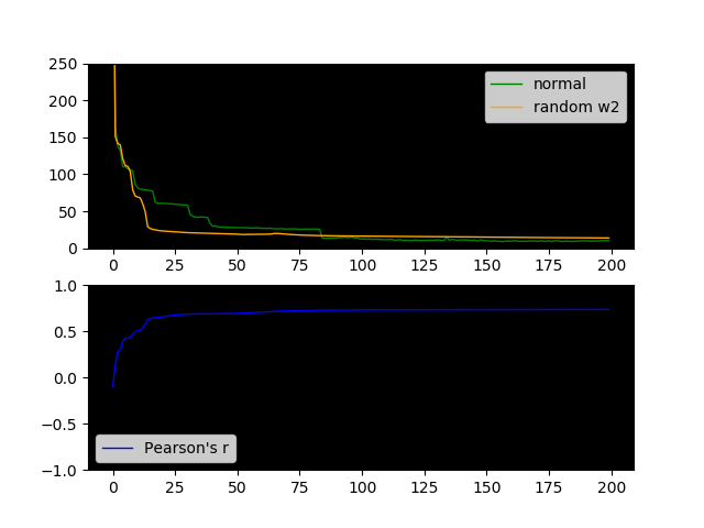
You can see that Pearson’s r increases as loss decreases, and it usually hovers around 0.75±0.05 by the end of the training. So there is some truth to my hypothesis. How much truth? r = 0.75 you could say!

More testing

To further test my hypothesis, I came up with an extreme case of it. I decided to predetermine w2_feedback, but not with normally distributed random numbers. This time, each neuron in the hidden layer should only have one weight in w2_feedback of value 1. w2_feedback is kept constant like before. Meaning each neuron in the hidden layer only receives \(\delta \) from one output neuron rather than all 10. That means if we have 20 hidden unit and 10 output units, each output unit has exactly 2 feedback weights + a bias. Here is the result:

hidden units	training set size	test set size	avg. accuracy w/ normal Backprop	avg. accuracy w/ random feedback Backprop	t-test p value	# of runs
20	50k	10k	93.1%	93.9%	0.007	30

Surprisingly again, not only did the network perform just as well as regular backprop (even slightly better), it worked even better than the random w2_feedback. If this scales to larger networks and other topologies it could potentially save a lot of computation resource. Here the amount of backprop computation from output to hidden layer was reduced by a factor of 20! Perhaps I’ll explore this in a future post.

Here is the code again; Happy hacking!